Summary

This post presents a method for constructing a statistical model to represent the wind environment at some particular site. The wind speed and direction record from the ‘Wellington Aero’ meteorological station is used for this analysis but the method should be generally applicable. This model will be used in Part 3 of this series to describe the reference site and scaled to generate local wind environments.

Wind history statistics and the wind rose

Wind history statistics describe the typical distribution of the wind speed and wind direction at a particular site. This information can be presented graphically as a wind rose plot and is generated from a meteorological record of wind speed and direction data.

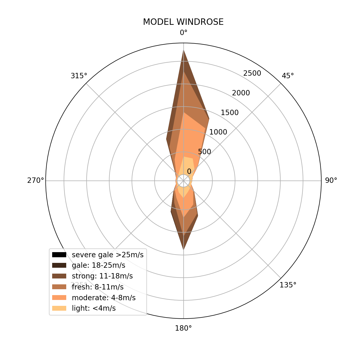
For example, the plot below shows the wind rose at the ‘Wellington Aero meteorological station’. This has been computed from a 13 year record of hourly averaged wind measurements taken at the airport site. The plot shows that the typical wind directions are either northerly or southerly. More specifically, the winds are typically directed in the NNE to NNW segment or the SSE to SSW segment. These directions account for the vast majority of the observational record.

The color scaling of the plot shows the distribution of wind speeds for each direction ranging from light (<4m/s) to strong (11-18m/s). Gale wind speeds have been only occasionally recorded at this site and are not apparent in this visualization.

The wind rose is generated using the matplotlib.pyplot package. The plotting function is given below.

def plotwindRose(data):
    fig = plt.figure(figsize=(7,7))
    fig.clf()
       
    # build windrose drom vel, dirn data
    ax = plt.subplot(111, projection='polar')
    cmap = cm.get_cmap('copper')
    speedbins=np.array([50, 25, 18, 11, 8, 4])
    speedlegend=['severe gale >25m/s', 'gale: 18-25m/s','strong: 11-18m/s','fresh: 8-11m/s','moderate: 4-8m/s','light: <4m/s']
    angles=22.5*np.linspace(0,16,17)
    angbins = (22.5*np.linspace(0,16,17)-11.25)

    vel=data[:,1]
    theta=data[:,0]
    
    inds = np.digitize(theta, angbins) # indices matched with angular bins
    for a,speed in enumerate(speedbins):
        y=[]
        for idx in 1+np.arange(len(angbins)-1): # go through angular bins
            bindata=vel[inds==idx] # select velocities for angular bin
            y.append(len(bindata[bindata<speed])) # count number of velociies at threshold 
        y.append(y[0])  # wrap around end
        y=np.array(y)
        ax.fill_between(angles/180*np.pi,0,y,facecolor=cmap(float(a)/(len(speedbins)-1)))
        
    ax.legend(speedlegend,loc='lower left',fontsize=10)
    ax.set_theta_zero_location("N")
    ax.set_theta_direction(-1)
    ax.set_rlabel_position(30)
    ax.set_title('WINDROSE')

A wind rose is a very useful climatological summary of a particular site. It could be used for making decisions about orientations of new buildings, expected wind loadings on structures or the sensibility of an outdoor picnic seat.

Statical modeling

The reference site used for this analysis is the ‘Wellington Aero’ Meteorological station located on the western site of the runway.There is a long observation record for this site which is publicly accessible through the CliFlo portal. From this the hourly averaged surface wind record was extracted the for the period of June 2000 - January 2013.

This is a huge observational record and it is beneficial to represent it by a statistical model. Wind speed distributions are typically represented with a Weibull distribution.

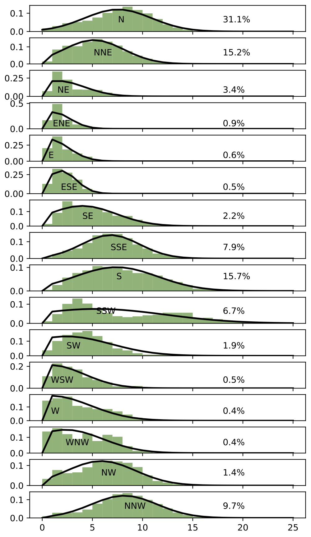
The wind record was divided into 16 different wind direction bins (N, NNE, NE, …) and then a Weilbull fit was performed for each of these using the scipy.stats.weibull_min function. This returns a wind speed probability distribution function v(c,loc,scale). The results of this are shown in the plot below where the bars represent the observational data and the solid line shows the distribution fit for each wind direction. The occurrence of each wind direction f is given on the right of a plot as a percentage.

By eye, the Weibull distribution does a good job of describing the data. The obvious exception is the SSW wind speed distribution which is almost bi-modal - however, even in this case the wind speeds are well described at the upper and lower limits by the Weibull fit. This wind directions has only a 7% occurrence and so this error seems tolerable

The statistical model to describe the sites wind speed and direction data W is: $\begin{align*} & W = \sum_{i=N}^S\left(v(c_i,loc_i,scale_i)f_i,\Theta(i-1,i+1)\right) \end{align*}$

The summation indicates the addition for all wind directions and $\Theta(i-1,i+1)$ represents random directions in each wind direction bin. E.g. for the northerly bin, the direction angles are randomly distributed between -11.25 and 11.25 degrees bearing.

Random variates can then be generated computationally using the function below. This generates 1 years worth of wind data (8760 hours).

def generateWindData(windModel):
    dirn=windModel['directions']
    angbins=windModel['angbins']
    
    W=[0,0] #initialise array (remove entry later)
    for a,w in enumerate(dirn):
        # get distribution parameters
        dists= windModel[w] 
        (c, loc, scale) = dists[0:3]
        occurrence=dists[3]
        # generate windspeeds
        vel=weibull_min.rvs(c, loc, scale, size=int(occurrence*8760))
        # gernate wind directions (random in angle bin)
        theta=angbins[a]+(angbins[a+1]-angbins[a])*np.random.random(size=int(dists[3]*8760))
        
        #wrap around correction for angles near N
        theta[theta>360]-=360
        theta[theta<angbins[0]]+=360
        W=np.vstack((W,(np.vstack((theta,vel)).T)))
    
    W=W[1:,:] # drop initialise entry
    return (W)

The quality of the statistical model can be well judged by comparing the observational ‘raw’ wind record against the model. This is shown below. The distribution of velocities and directions is very similar for the two plots. The scaling for the raw data is different because there is a 16 year record whereas the model is normalised for 1 year. The statistical model looks like a very good approximation.

Actual	Model

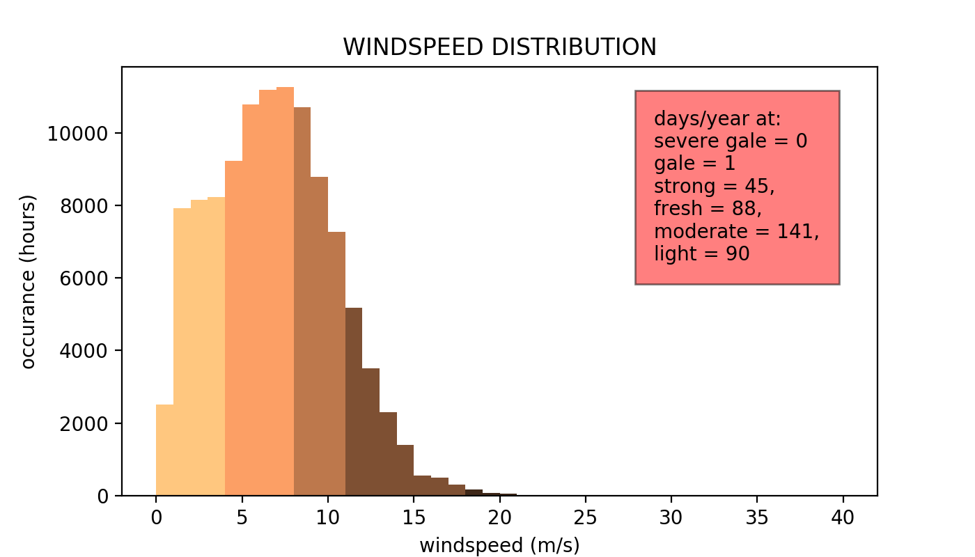
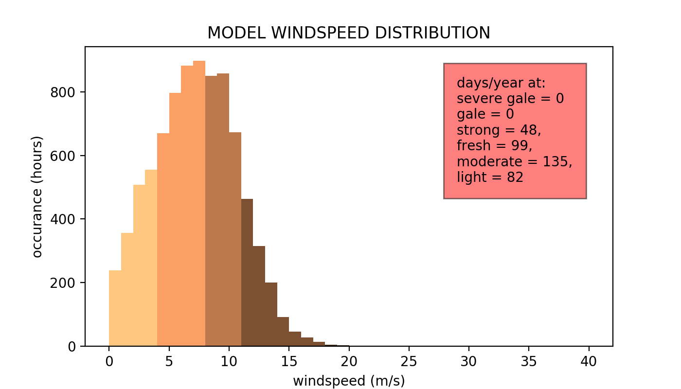
A further comparison can be made by ignoring the direction data and comparing only the distribution of wind speeds. This is shown below for the two cases. The model misses some of the fine detail seen in the record or low wind velocities. However the model gives good agreement for all other wind speeds.

Actual	Model

These plots also show statistics summarising the total day’s per year where wind categories occur. This is a good human relatable scale for the data. Again the model gives good agreement to observational record.

Conclusions

The wind record for the Wellington Aero station is well represented by a statiscal model comprising of Weibull distributions summed and weighted for different wind directions. This formulation gives a succinct represent of the local wind environment and will be a useful input for part 3 of this project where we look to scale a reference wind environment by a regional model to predict local wind environments.