Summary

This post describes the construction of a Computational Fluid Dynamic (CFD) model of the Wellington region which gives local detail of the wind flow around topography. This model will be used in Part 3 of this blog series to scale the reference site wind distribution and generate local wind environment statistics.

What’s CFD?

The wind flow across some region can be modeled using the technique of computational fluid dynamics (CFD). This method calculates how the wind flows through space and around obstructions. It like a virtual wind tunnel and provided the model is correctly constructed, it should reproduce the local wind effects caused by the terrain. CFD simulations are quite complicated beasts and I will only try here to give a quick overview of the process.

Building a CFD model

The first step in constructing a CFD model is to define the relevant physics which must be solved for. For this work is was assumed that the lower atmosphere could be modeled as an incompressible homogeneous layer. The Navier Stokes equations, which describe fluid dynamics, will be solved in their Reynolds-averaged forumulation to give a steady state solution of velocity, pressure, and the turbulent kinetic energy, rate of dissipation and viscosity for discrete volumes within the model. The OpenFoam CFD package was used for this simulation.

The model extent must next be defined. For this work the basic model size was a rectangle 12km x 12km x 960m high. This work could be easily scaled up for larger regional models - however the simulation is computationally intense and larger models would take longer to solve.

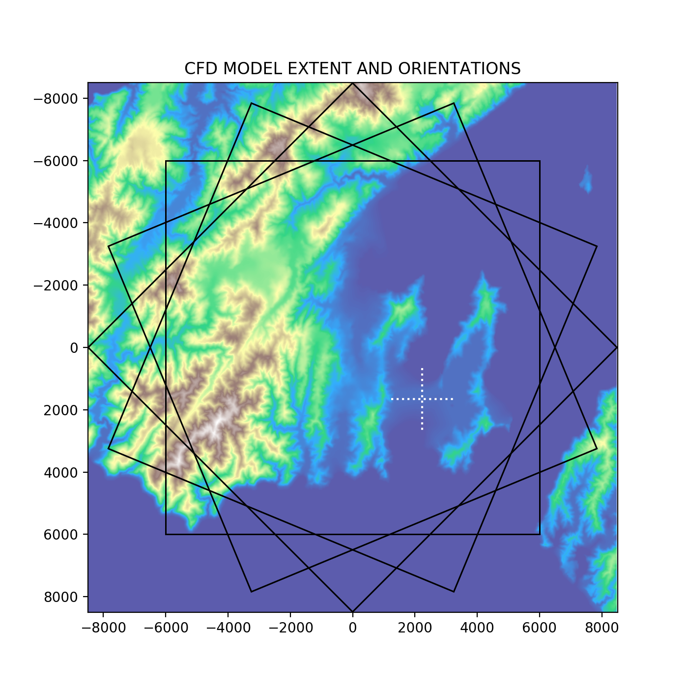
The model was centered on Wellington city and rotated through 16 orientations for wind directions N, NNE, NE etc. The projections are shown on the map image below. The white cross is the location of the Wellington Aero reference site which was used in the first post of this series.

The bottom boundary of the model is the terrain - the data source for this is the [LINZ 8m Digital Elevation Model] (https://data.linz.govt.nz/layer/51768-nz-8m-digital-elevation-model-2012/). To work with the CFD software this elevation model needs to be converted to a stl standard 3d model file. There is a Python script available for doing this provided here. In the model this ground layer has an imposed no-slip boundary condition - this means the boundary velocity is zero. This same no-slip boundary condition is imposed for the top and sides of the model. For the inlet a log wind profile normalized to 10m/s is applied and the outlet is set at zero pressure. The absolute velocities in the model are not particularly import because the data will only be used for scaling relative to a reference site.

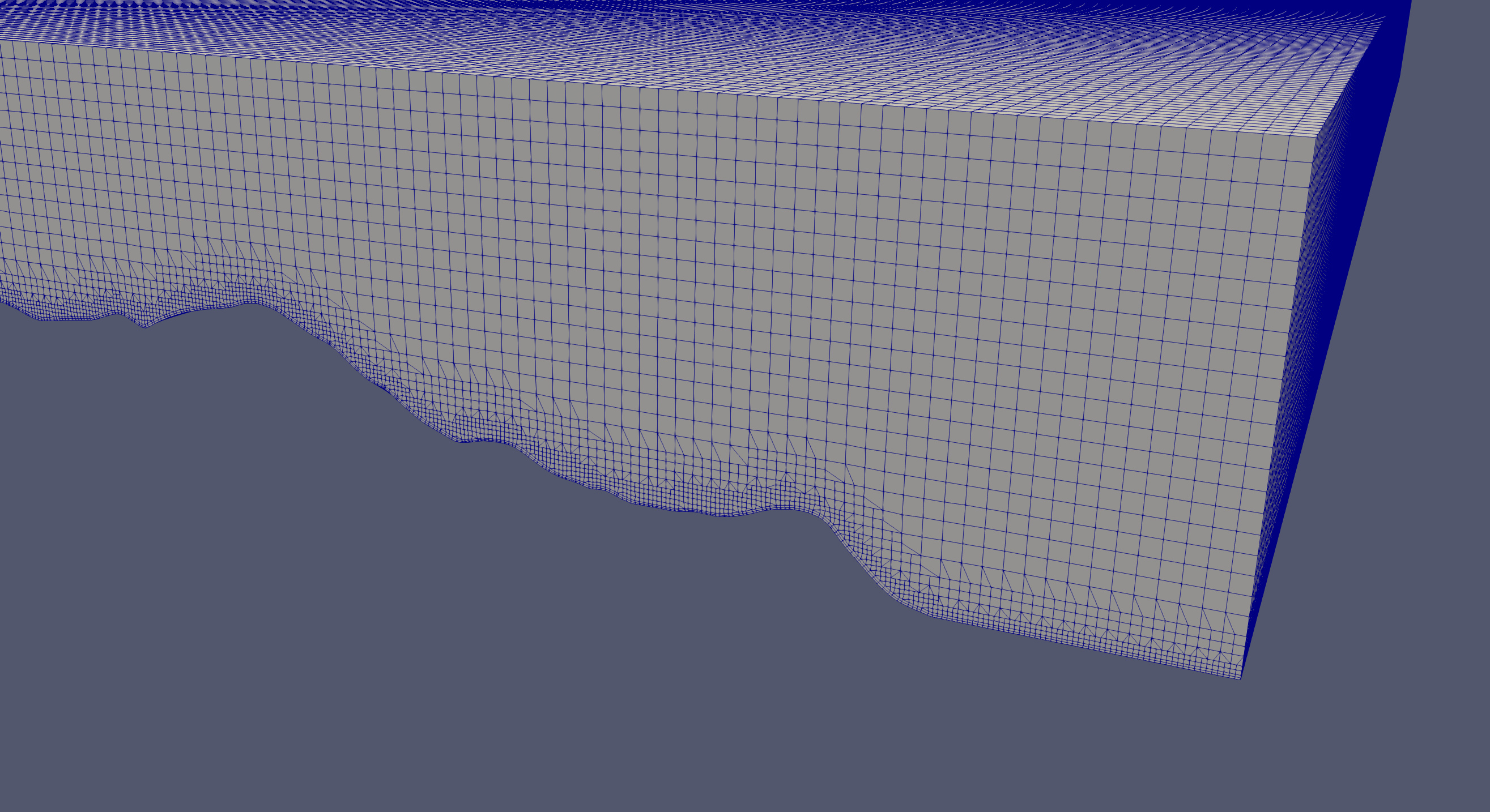
The model domain is then discretized into what is mostly a hexahedral mesh using the snappyHexMesh utility - this tool is included in the openfoam installation. The base mesh has a 40m resolution but refines down to 10m as it approaches the terrain surface. The mesh completes with two layers aligned to the boundary surface. The mesh is approximately 20 million cells in size.

The CFD models require quite a bit of computational muscle to complete. For this work the simulations were performed on an AWS c5 4xlarge instance - this virtual machine allows for parallel processing across 8 cores and has ample memory for the model size. The model solutions converged after approximately 1000 iterations (2 hours).

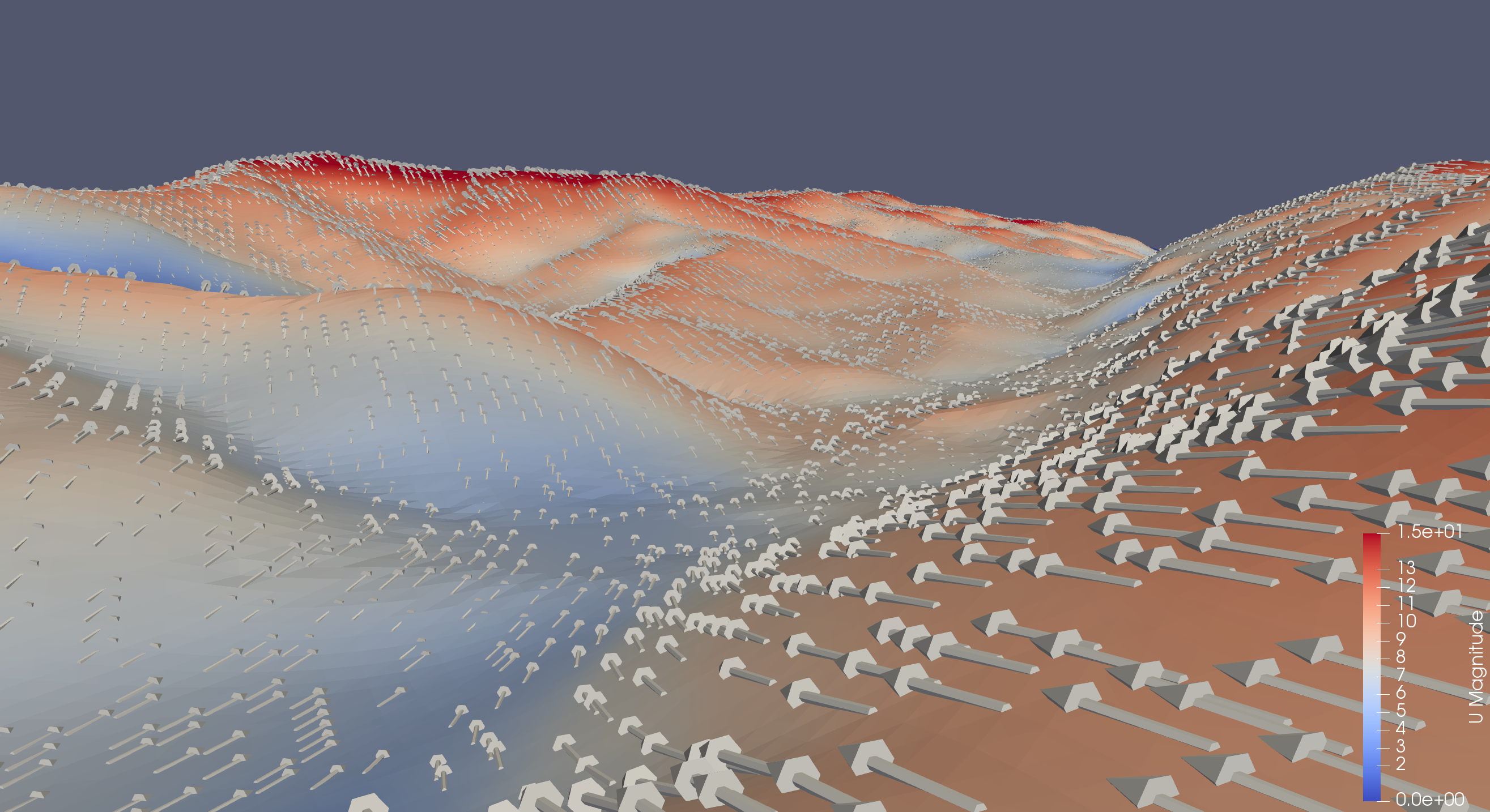
For this work we are only interested in wind speeds near the ground surface and so we can take a slice from the full 3D solution. To avoid boundary defects it is important to sample the solution from a cell which is not nearest the boundary. For this work velocity slices at a height of 20m above the surface are sampled using the paraview (a visualization and analysis tool). One such slice is shown below - the color scale gives the magnitude of the velocity and the arrows give the vector direction. Regional effects are evident. Directional changes are shown by the arrows and the wind speeds are highest on the hill top.

The surface slices were exported from paraview for the 16 different wind directions. From these datasets Python interpolation objects were generated which give bivariate spline approximations to the surface velocity magnitude and direction. This were generated using the scipy package class interpolate.RectBivariateSpline class. This then gives for each wind direction the functions $fv_i(x,y)$ and $f\theta_i(x,y)$ which described the velocity magnitude and direction at location coordinates x,y. These functions will be used in part 3 of this to scale reference site observations to a wind expectancy at any site.